Simple Strategies That Made Money: Three Windows in Market History

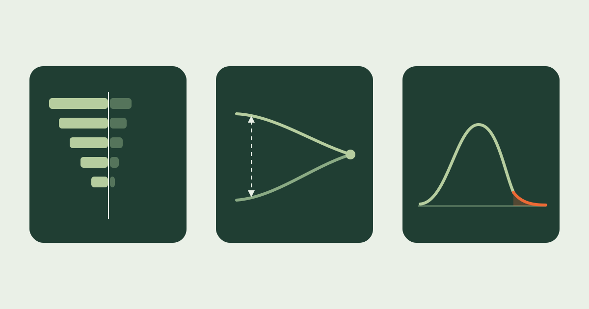
The strategy that fits in one paragraph

Most people picture a profitable trading strategy as something elaborate: many signals, a large model, a research team behind it. Several of the most profitable trades of the past twenty years were not like that at all. They fit on an index card, and the people running them would have explained the idea over coffee without much fear that you would take it from them.

The hard part was rarely the mathematics. It was being in the right market early, paying costs small enough to leave something behind, and building something that kept running. This article walks through three of those windows—one from traditional markets, one from crypto in 2020, one from short-dated prediction markets—and then asks what remains once a window narrows.

None of it is a recommendation or a claim about what is available today. Every window described here closed, or is closing, as participants arrived. Read them as history with a practical moral.

The book leaned, and that was the trade

Twenty years ago, in equities and futures, one sentence was worth a great deal: compare the resting quantity at the best bid with the quantity at the best offer, and lean toward the heavier side. Cont, Kukanov, and Stoikov formalized the version that reached the literature—over short horizons, price changes in their sample move roughly linearly with the imbalance between buy and sell order flow at the top of the book.

Those quantities were on every screen. The scarce ingredient was never the signal; it was the ability to act on it—a fast feed handler, a short physical path to the matching engine, and a place near the front of the queue. Budish, Cramton, and Shim describe what that competition became: a race measured in microseconds, a mechanical contest in which the fastest participant collects and the others pay.

The signal did not stop working. It became expensive to harvest. A handful of firms still monetize book and taker-flow imbalance today, at horizons of milliseconds, because they own the infrastructure that reaching it requires. That is the ordinary life cycle of a simple idea: it stops being enough when the cost of acting on it grows to meet what it produces.

Research: the price impact of order book events — Cont, Kukanov, and StoikovResearch: the high-frequency trading arms race — Budish, Cramton, and Shim

2020: the same coin at two prices

Crypto in 2020 offered a different kind of simplicity. A perpetual future and the spot market quote the same asset. When the perpetual traded above spot, you could buy the coin, sell the perpetual against it, and collect the funding that longs paid shorts for as long as the gap persisted. No forecast of the price was needed; the position was close to flat by construction.

Makarov and Schoar documented how large and persistent price deviations across crypto venues had been in the preceding years—differences far beyond what equity markets tolerate, lasting long enough to trade deliberately. The arithmetic required to act on them is secondary-school arithmetic.

The work was somewhere else entirely. Two exchange integrations, two balances, transfers between them, a monitor that knew whether both legs were still open, margin management on the short leg, and an explicit rule for what to do when funding turned negative and stayed there. The trade did not need a better model. It needed a system that did not break at three in the morning.

A hedged position is not a riskless one, and it is worth saying so plainly. Basis can widen before it converges, funding can invert for weeks, a transfer can fail at the worst moment, and the venue is itself a counterparty. Those risks are what the carry is paying for.

Research: trading and arbitrage in cryptocurrency markets — Makarov and Schoar

The first months of crypto UP/DOWN markets

Short-dated crypto prediction markets ask a narrow question: will the settlement price be at or above a given level at the end of the hour, the fifteen minutes, or the minute? That question has a textbook answer. Model the price as a random walk, standardize the distance to the level by the volatility over the time remaining, and read the probability off the normal distribution.

In the early months of such markets, quotes could sit a long way from that estimate. It was most visible far from the money and close to expiry, where a contract the model values at a fraction of a cent still trades for several cents because someone wants the lottery ticket. A strategy that did nothing but wait for a large gap and then send an immediate-or-cancel order—expecting no fill most of the time—did not need to be right often. It needed the gap to be wide enough to survive costs, and it needed the discipline to refuse everything else.

One small refinement changes more than any amount of added complexity: replace the normal distribution with the empirical distribution of recent returns. Crypto returns have heavier tails than a Gaussian—heavy-tailed fluctuations are among the oldest stylized facts in the literature. A Gaussian model therefore understates the chance of a large move, and it is most overconfident exactly where the far-from-the-money contracts live. Depending on the side you are taking, that correction removes trades that looked free and keeps ones that looked too expensive.

This is the part to be careful about. We are describing a window, not a standing opportunity. Whether such gaps exist in a particular market today, in a size worth trading, after fees and adverse selection, is an empirical question whose answer moves. The honest version of this strategy arrives with a measurement attached, not a story.

Research: heavy-tailed fluctuations in financial markets — Gopikrishnan, Plerou, and colleagues

Why windows close, and what survives

Each of these narrowed the same way. Participants arrive, quotes tighten, and the cost of trading does not fall as quickly as the edge does. On short-dated contracts the arithmetic is unforgiving: one cent of edge on a fifty-cent share is two percent of the amount at risk, and a round trip costing about one percent takes half of it before you allow for the model being wrong.

What tends to survive is the simple idea with a constraint attached—a market that is awkward to reach, a size too small for a large firm to bother with, a horizon nobody is watching, or a settlement rule that takes real work to reconstruct. The edge migrates from the idea to the effort around it.

The other thing that survives is measurement. In every one of these windows, the people who did well were not the ones with the cleverest hypothesis. They were the ones who kept checking whether it was still true this week.

Three windows, three building blocks

All three ideas exist in Quant Fun as blocks you can place on a canvas. Each carries the parts that are tedious to build and easy to get wrong: feed handling, venue semantics, settlement definitions, and checks for stale or missing data.

A strategy can be one condition and one action. A reasonable first experiment on a fifteen-minute crypto market is four nodes long: enough time remaining, a model edge over the best ask, a sensible price range, then an IOC. More elaborate strategies are equally possible—several signals arranged across entry, cancel, and exit. The canvas does not require complexity before it takes an idea seriously.

• Order-book imbalance: Polymarket, Binance, and Lighter book-imbalance conditions, plus Taker flow imbalance for buyer- versus seller-initiated trades over a chosen lookback.
• Basis and carry: Funding rate, Spot or TWAP basis, and the cross-exchange setup behind Executable cross minus rolling basis.
• UP/DOWN pricing: Random-walk simulation for the model probability, and Random-walk mispricing to compare that probability against the price you can actually trade.
• Execution: IOC for an immediate attempt, Post-only for a resting quote, and order-age and price-distance conditions for deciding when to give up on one.

Simple is a starting point, not a conclusion

Simple does not mean unexamined. The difference between a simple strategy that made money and one that quietly lost it is usually the measurement around it: a replay with realistic fills and fees, a look at what the price did right after each fill, and results from hours you did not choose in advance.

Watch the history you are testing on as well. A short archive and a wide parameter search will hand you an excellent-looking result that is only luck. The remedies are a longer horizon, fewer variants, and an out-of-sample period you commit to before you look at it.

That is why the studio exists: to keep the distance between “I can explain this in a paragraph” and “I have tested it and it is running” as short as it can honestly be. The windows above are not open invitations. They are evidence that an idea worth trading often fits in a paragraph—and that the work is proving which paragraph.